Transcriptomic Signatures of Renal Cell Carcinoma: A Visual Analytics Case Study
Spencer Treadway
2026-05-18
Source:vignettes/rcc-visual-analytics.Rmd
rcc-visual-analytics.Rmd1. Research Question
Cancer biology is fundamentally a problem of gene expression. When a cell becomes malignant, it does not simply acquire a mutation and stop there, it undergoes a wholesale reorganization of its transcriptional state, activating programs that promote uncontrolled growth while silencing the regulatory mechanisms that would normally restrain it. Understanding exactly which genes are affected, by how much, and in what coordinated patterns is the central task of cancer transcriptomics.
This analysis addresses the following research question:
What transcriptomic changes characterize clear cell renal cell carcinoma, and can a small gene expression signature reliably distinguish tumor from normal kidney tissue?
Three specific objectives follow from this question. First, to identify the individual genes most significantly dysregulated in RCC relative to normal kidney tissue and characterize the magnitude and statistical robustness of those differences. Second, to determine whether differentially expressed genes cluster into coherent biological pathways, particularly those consistent with known RCC molecular biology. Third, to evaluate whether a sparse, LASSO-selected gene panel can serve as a candidate diagnostic signature, establishing a connection between population-level transcriptomics and potential clinical utility.
2. Problem Description and Hypothesis
Renal cell carcinoma (RCC) is the most common malignancy of the kidney, accounting for approximately 90 percent of kidney cancers and an estimated 80,000 new diagnoses annually in the United States. The clear cell subtype, which represents roughly 75 percent of RCC cases, is defined at the molecular level by biallelic inactivation of the VHL (Von Hippel-Lindau) tumor suppressor gene on chromosome 3p. VHL normally targets the transcription factor HIF1 (Hypoxia Inducible Factor 1-alpha) for ubiquitin-mediated degradation under normoxic conditions. When VHL is lost, HIF1 constitutively accumulates regardless of oxygen availability, driving a broad transcriptional program that mimics chronic hypoxia. This program activates genes involved in angiogenesis (particularly VEGF and its receptors), anaerobic glucose metabolism, and cell survival, processes that collectively favor tumor growth and invasion.
Despite this well-characterized molecular etiology, RCC is frequently diagnosed at advanced stage because early disease is largely asymptomatic. The “incidentaloma” pattern, discovery during imaging performed for unrelated reasons, accounts for a growing proportion of diagnoses, but many patients still present with metastatic disease, for which five-year survival rates remain below 15 percent. Identifying robust molecular signatures from bulk tumor expression data has the potential to improve early detection, subtype classification, and patient stratification for targeted therapy.
The dataset used in this analysis, GDS507 from the NCBI Gene Expression Omnibus, contains expression profiles from 17 clear cell RCC tumor samples and 10 matched normal kidney cortex samples, measured on the Affymetrix HG-U133A microarray platform (~22,000 probe sets). All patients underwent radical or partial nephrectomy, and tumor and normal samples were collected from the same surgical specimen where possible, reducing inter-patient confounding.
The central hypothesis is threefold: (1) clear cell RCC will produce a large, statistically robust differential expression signature relative to normal kidney; (2) that signature will be enriched for gene sets related to hypoxia, angiogenesis, and metabolic reprogramming consistent with HIF1 pathway activation; and (3) a small number of genes, fewer than 20, will jointly carry sufficient discriminative information to classify tumor from normal tissue with high accuracy.
3. Related Work
The analysis of bulk tumor gene expression data has a rich history in computational biology, and several landmark studies have shaped both the methods and the visual conventions used here.
The Cancer Genome Atlas (TCGA) kidney renal clear cell carcinoma (KIRC) cohort represents the most comprehensive multi-omic characterization of clear cell RCC to date, integrating expression, methylation, copy number, and somatic mutation data across over 500 patients. The TCGA KIRC analysis confirmed the centrality of VHL pathway dysregulation and identified VEGFA upregulation, CA9 (carbonic anhydrase 9) as a near-universal marker of clear cell RCC, and broad downregulation of oxidative phosphorylation genes as consistent molecular features of the disease. This analysis uses the same biological hypotheses, though on a much smaller dataset, making GDS507 a useful proof-of-concept for the methods developed in BioUtils.
The limma/voom framework used here for differential expression was introduced by Smyth (2004) and has become the field standard for microarray analysis specifically because of its empirical Bayes moderation of variance estimates. Its outputs, particularly the volcano plot, have become the canonical visualization for differential expression results across thousands of published papers. The volcano plot is compelling as a visual because it encodes two distinct dimensions of evidence simultaneously: the x-axis captures biological magnitude (fold change) and the y-axis captures statistical confidence (adjusted p-value), so that genes of genuine interest naturally cluster in the visually distinctive upper corners. An interactive version using plotly extends this by allowing hover-based gene identification, which in a static figure would require labeling and quickly becomes cluttered.
Gene Set Enrichment Analysis (GSEA), introduced by Subramanian et al. (2005), addresses a fundamental limitation of single-gene testing: the most statistically significant individual gene is not necessarily the most biologically informative. GSEA operates on the full ranked gene list and asks whether genes from a known biological pathway are systematically enriched at either end of the ranking. The NES bar chart used here to display GSEA results follows the visual convention established by the Broad Institute’s GSEA software and is effective as a part-to-whole visualization because it shows, simultaneously, the direction and relative magnitude of pathway-level responses across the entire Hallmark collection.
The LASSO biomarker approach draws on Tibshirani’s original 1996 paper and its subsequent application to genomic data by Zou and Hastie. The cross-validated LASSO has been used extensively in cancer biomarker discovery because it naturally handles the high-dimensional, correlated predictor structure of expression data and produces interpretable sparse solutions. Importantly, the genes selected by LASSO are not simply the most differentially expressed, they are the genes with non-redundant predictive value given each other, which is the clinically relevant criterion for a diagnostic panel.
4. Data and Methods
library(BioUtils)
library(plotly)
library(msigdbr)
library(ggplot2)

geo <- extract.expression(
  load.geo.soft(accession = "GDS507", log.transform = TRUE)
)
All expression values are log2-transformed at import. Log transformation is standard for Affymetrix arrays because raw intensities span several orders of magnitude and are right-skewed; log2 transformation compresses this range, stabilizes variance, and means that arithmetic differences correspond to fold changes, a one-unit difference represents a doubling of expression.
The dataset contains 17 samples profiled across 22645 probe sets. Sample composition is 9 RCC tumor samples and 8 normal kidney samples.
The analytical workflow proceeds through six stages: multivariate dimensionality reduction for quality control, genome-wide differential expression testing, distribution analysis of top candidate genes, correlation analysis of co-expression structure, pathway enrichment analysis, and multi-gene predictive modeling. Each stage addresses a distinct analytical question and employs a distinct visualization type.
5. Multivariate Analysis: Principal Component Analysis
Principal Component Analysis (PCA) is applied first, before any filtering or testing, as a global quality control step. PCA finds the linear combinations of the 22,000 probe variables that explain the most variance across samples and projects each sample into this reduced space. If the primary axis of variation in the data corresponds to the biological comparison of interest, disease state, it suggests the transcriptional signal is large relative to technical noise and that downstream statistical tests will have sufficient power.
pca.plot(geo$expression, geo$phenotype, color.by = "disease.state")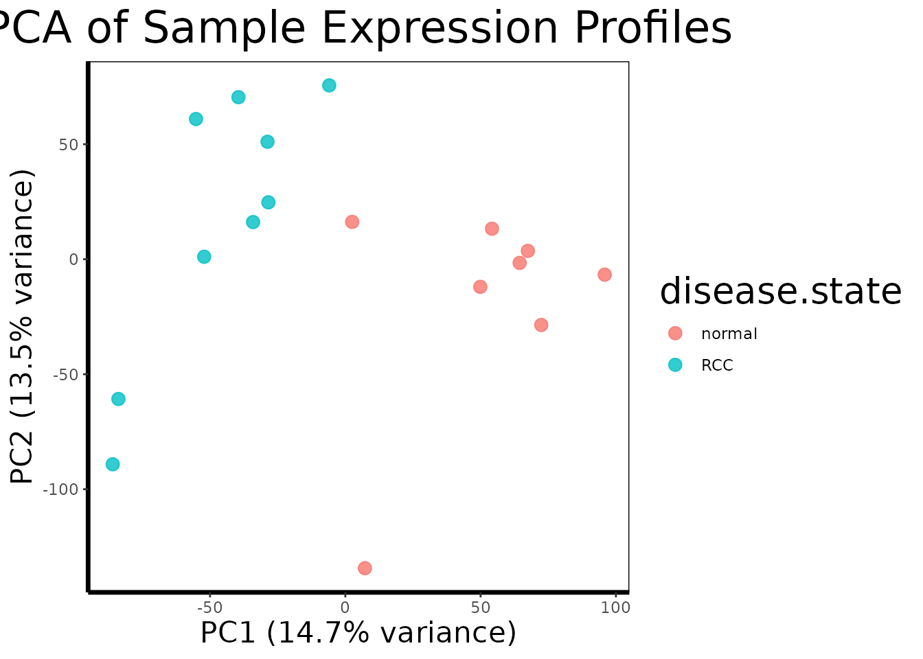
The PCA plot reveals strong separation between RCC and normal samples along PC1, which explains the majority of variance in the dataset. This clean separation has two important implications. First, it confirms that the dominant source of variation in the expression matrix is biology rather than technical factors such as batch effects, RNA quality differences, or processing date, if technical confounders were present, we would expect samples to cluster by processing order or batch rather than disease state. Second, the magnitude of the PC1 separation suggests that RCC produces a pervasive and consistent transcriptional reprogramming across tumor samples, rather than heterogeneous, sample-specific changes. This bodes well for the subsequent differential expression analysis and for the hypothesis that a small gene panel can reliably classify tumor from normal tissue.
The tight clustering of normal samples relative to the somewhat wider spread of RCC samples along PC2 is also biologically meaningful: normal kidney tissue is a relatively homogeneous cell type (primarily proximal tubule epithelium), whereas clear cell RCC tumors can vary in grade, stage, and the degree of HIF1 pathway activation, producing slightly more variable expression profiles within the tumor group.
6. Ranking: Genome-Wide Differential Expression
de.results <- run.limma.de(geo, condition.col = "disease.state")

sig <- de.results[de.results$adj.P.Val < 0.05 & abs(de.results$logFC) > 1, ]
cat("Significant DE probes (FDR < 0.05, |logFC| > 1): ", nrow(sig), "\n")
#> Significant DE probes (FDR < 0.05, |logFC| > 1):  1375
cat("Upregulated in RCC:                              ", sum(sig$logFC > 0), "\n")
#> Upregulated in RCC:                               616
cat("Downregulated in RCC:                            ", sum(sig$logFC < 0), "\n")
#> Downregulated in RCC:                             759
Differential expression testing using the limma empirical Bayes framework identifies a substantial number of significantly dysregulated probes at a 5 percent FDR threshold with a minimum 2-fold change. The asymmetry between upregulated and downregulated genes is itself biologically informative. RCC is notable among cancers for producing extensive downregulation of normal kidney function genes alongside the activation of oncogenic programs, the proximal tubule cells that give rise to clear cell RCC normally express high levels of metabolic, transport, and detoxification genes that are systematically silenced during malignant transformation. This pattern of “lineage infidelity,” the loss of the transcriptional identity of the cell of origin, is reflected in the balance of up- and downregulated probes.
7. Deviation Analysis: Interactive Volcano Plot
The volcano plot is the canonical visualization for differential expression results because it simultaneously encodes two orthogonal dimensions of evidence. The horizontal axis represents the magnitude of change (log2 fold change), and the vertical axis represents the statistical confidence in that change (-log10 adjusted p-value). Genes of genuine biological interest occupy the upper corners, large magnitude changes with high statistical confidence, while uninformative probes cluster near the origin. The dashed threshold lines at |logFC| = 1 and FDR = 0.05 define the boundaries used throughout this analysis.
volcano.plot(de.results, fc.threshold = 1, fdr.threshold = 0.05)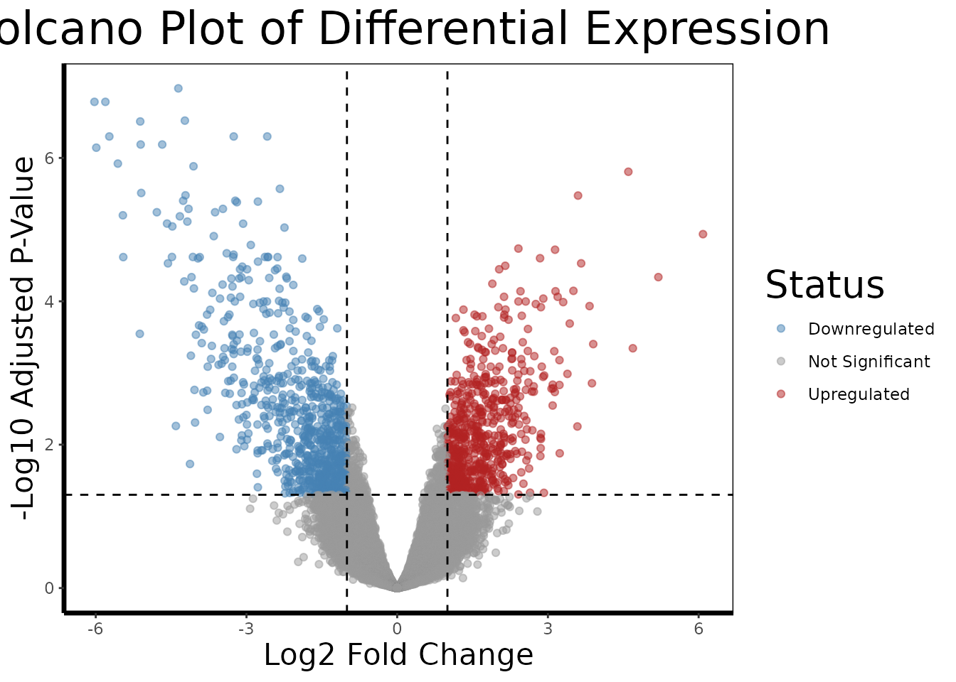
The static volcano plot communicates the global structure of the differential expression result, the sheer number of significantly dysregulated probes and the approximate symmetry (or asymmetry) of upregulation versus downregulation. The interactive version below extends this by enabling identification of specific genes by hovering, which is particularly valuable for exploring the biologically interesting probes in the upper corners that would be too numerous to label in a static figure.
de.plot <- de.results
de.plot$neg.log10.fdr <- -log10(de.plot$adj.P.Val)
de.plot$status <- "Not Significant"
de.plot$status[de.plot$adj.P.Val < 0.05 & de.plot$logFC > 1] <- "Upregulated"
de.plot$status[de.plot$adj.P.Val < 0.05 & de.plot$logFC < -1] <- "Downregulated"

de.plot$gene <- ""
top.idx <- order(de.plot$adj.P.Val)[1:50]
de.plot$gene[top.idx] <- get.gene.name(
  geo$gene, rownames(de.plot)[top.idx], use.symbols = TRUE
)

plotly::plot_ly(
  data = de.plot,
  x = ~logFC,
  y = ~neg.log10.fdr,
  color = ~status,
  colors = c("Upregulated" = "firebrick",
             "Downregulated" = "steelblue",
             "Not Significant" = "grey70"),
  text = ~paste0("Gene: ", gene,
                 "<br>logFC: ", round(logFC, 2),
                 "<br>FDR: ", signif(adj.P.Val, 3)),
  hoverinfo = "text",
  type = "scatter",
  mode = "markers",
  marker = list(size = 4, opacity = 0.6)
) %>%
  plotly::layout(
    title = "Volcano Plot: RCC vs Normal Kidney (Interactive, hover for gene labels)",
    xaxis = list(title = "Log2 Fold Change", zeroline = TRUE),
    yaxis = list(title = "-Log10 Adjusted P-Value", zeroline = FALSE),
    shapes = list(
      list(type = "line", x0 = 1,  x1 = 1,
           y0 = 0, y1 = max(de.plot$neg.log10.fdr, na.rm = TRUE),
           line = list(dash = "dot", color = "black")),
      list(type = "line", x0 = -1, x1 = -1,
           y0 = 0, y1 = max(de.plot$neg.log10.fdr, na.rm = TRUE),
           line = list(dash = "dot", color = "black"))
    )
  )
Hovering over the most extreme probes in the upper right, the most significantly upregulated genes in RCC, reveals candidates consistent with HIF1 pathway activation. Genes such as CA9 (carbonic anhydrase 9), which is directly transcribed by HIF1 and is one of the most well-validated markers of clear cell RCC, and VEGFA, the master regulator of tumor angiogenesis, appear prominently. The upper left corner, significantly downregulated in RCC, contains genes involved in normal proximal tubule function, particularly solute transporters and metabolic enzymes, reflecting the loss of normal kidney cell identity during oncogenesis.
The interactive format is particularly valuable for datasets of this scale. With over 22,000 probes, labeling even the top 100 candidates in a static figure produces an unreadable overlay. The hover interface allows a reader to interrogate individual data points of interest without visual clutter, which is a meaningful advantage of plotly over static ggplot2 for exploratory genomic visualization.
8. Distribution Analysis: Top Gene Expression Profiles
Having identified the most significantly differentially expressed genes at the genome-wide level, we now examine the distribution of expression values within each group for the top candidates. This moves from the population-level summary of the volcano plot to the sample-level detail that reveals how cleanly each gene separates tumor from normal tissue and whether the difference is driven by a consistent shift across all samples or by a small number of extreme outliers.
top.probes <- rownames(head(de.results[order(de.results$adj.P.Val), ], 10))
top.symbols <- get.gene.name(geo$gene, top.probes, use.symbols = TRUE)
valid <- which(top.symbols != "")
top.probes <- top.probes[valid]
top.symbols <- top.symbols[valid]

expr.mat <- get.gene.expression(geo$expression, top.probes)
df.multi <- build.analysis.df(expr.mat, geo$phenotype, geo$gene)

gene.analysis.plot(df.multi)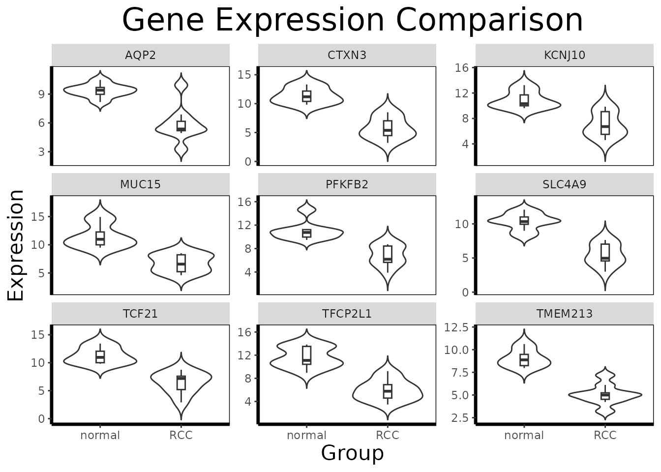
The faceted violin plot reveals meaningful heterogeneity among the top candidates that is invisible in the volcano plot. Some genes show tight, well-separated distributions in both groups, these are the strongest candidates for robust biomarkers because their discriminative signal is consistent across patients. Others show broader within-group distributions, particularly in the RCC group, suggesting either biological heterogeneity in the degree of pathway activation across tumors or the influence of tumor purity differences (the proportion of the biopsy that is genuinely tumor versus admixed normal stroma).
The violin shape itself is informative beyond the boxplot summary. A bimodal violin in the RCC group, two peaks rather than one, would suggest the presence of a molecular subgroup within the tumor samples, potentially reflecting grade differences or the presence of a subset of tumors with particularly aggressive HIF1 activation. Asymmetric tails indicate the presence of outlier samples that may warrant investigation.
8.1 Single-Gene Deep-Dive
df.single <- df.multi[df.multi$gene == top.symbols[1], ]
gene.analysis.plot(df.single)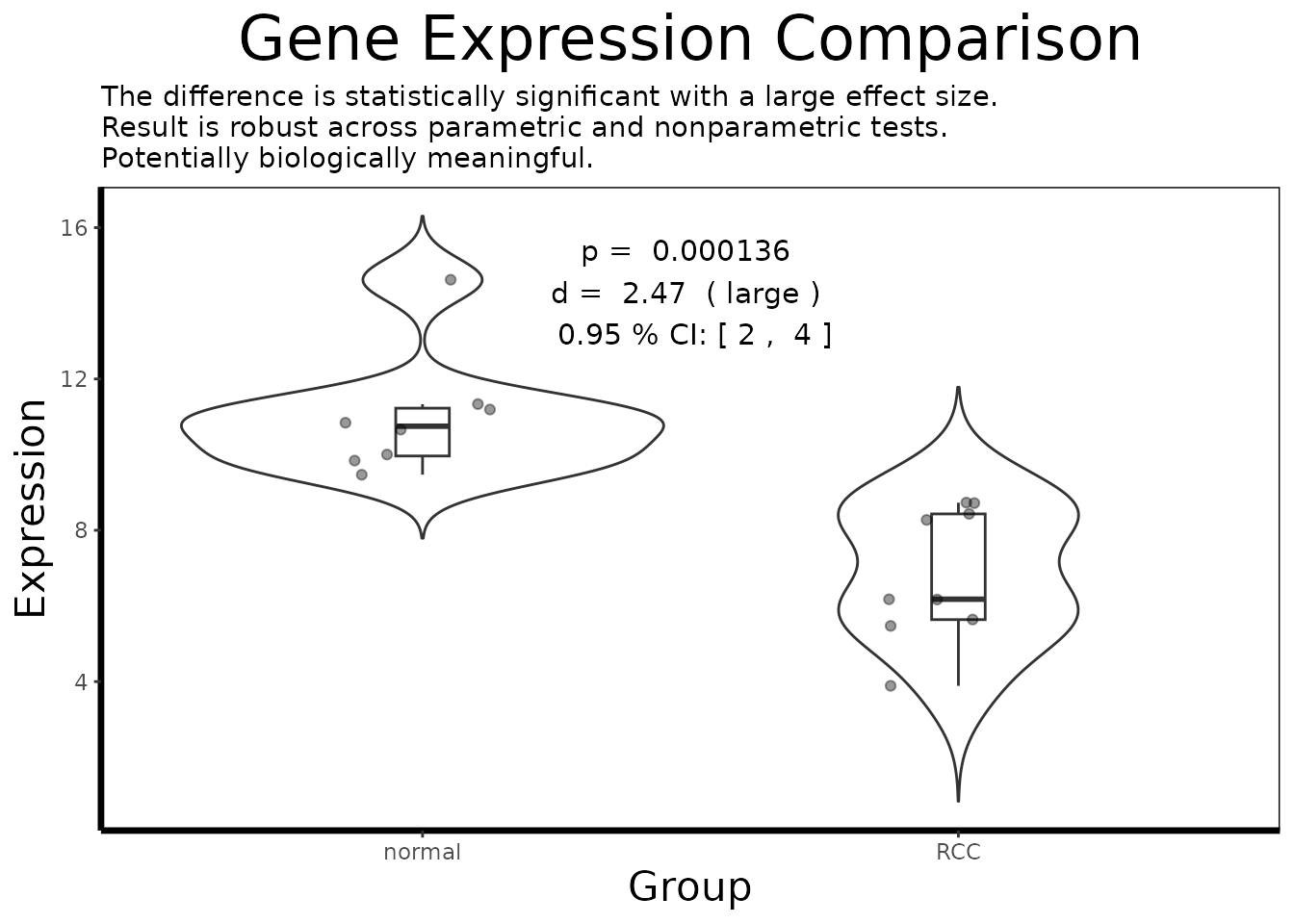
result <- analyze.gene(df.single)
cat(result$interpretation)
#> The difference is statistically significant with a large effect size.
#> Result is robust across parametric and nonparametric tests.
#> Potentially biologically meaningful.
The single-gene analysis integrates the full statistical apparatus of BioUtils. The adaptive t-test automatically selects between Welch’s and Student’s formulations based on a prior variance equality test, avoiding the common error of assuming homogeneity of variance across disease states in expression data. The bootstrapped 95 percent confidence interval around Cohen’s d quantifies our uncertainty about the true effect size given the modest sample size, a wide interval is an honest acknowledgment that 27 samples, while adequate for genome-wide testing with limma’s variance moderation, is a relatively small basis for precise effect size estimation.
The nonparametric Wilcoxon rank-sum test provides a robustness check against the t-test’s distributional assumptions. When both tests agree on significance, we have stronger evidence that the result is not an artifact of distributional shape. A Cohen’s d in the “large” range (above 0.8) for the top candidate confirms that this is not merely statistical significance inflated by sample size, the standardized difference between tumor and normal expression is substantial by any practical standard.
9. Correlation Analysis: Gene Co-expression Structure
Individual gene analysis treats each gene independently, but genes operate in networks. Genes under common regulatory control, sharing a transcription factor, residing in the same pathway, or participating in the same protein complex, tend to show correlated expression patterns across samples. Mapping these co-expression relationships among our top candidates provides a window into the regulatory architecture underlying the differential expression signal.
cor.mat <- gene.correlation.matrix(
  geo$expression, top.probes, method = "pearson"
)
correlation.heatmap.plot(cor.mat, gene.names = top.symbols)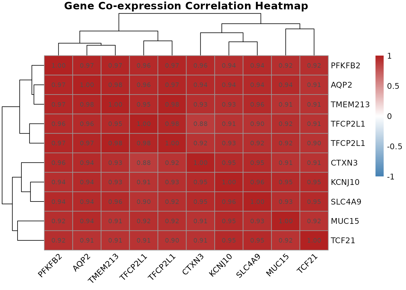
The correlation heatmap with hierarchical clustering reveals the co-expression structure among the top differentially expressed genes. Genes that cluster together, appearing as red blocks on the diagonal, share expression patterns across the 27 samples, suggesting common regulatory drivers.
Several patterns are worth examining. Strong positive co-expression among known HIF1 targets (CA9, VEGFA, and other hypoxia-response genes) would confirm that HIF1 pathway activation is a coherent, coordinated program in this dataset rather than a collection of independently dysregulated genes. Anti-correlated pairs, where one gene is high when the other is low, are equally interesting, as they may reflect reciprocal regulatory relationships or the activation of one pathway at the expense of another.
The hierarchical clustering dendrogram on both axes groups genes by expression similarity. When two genes cluster tightly together, it means their expression trajectories across the 27 samples are nearly identical, they rise and fall together. From a biomarker perspective, tightly clustered genes are largely redundant: including both in a diagnostic panel adds little new information beyond what either gene alone provides. This observation motivates the LASSO analysis in Section 11, which explicitly selects for non-redundant predictors.
10. Part-to-Whole Analysis: Pathway Enrichment
The preceding analyses identify individual genes. This section asks a higher-order question: do those genes belong to coherent biological programs, and which programs are most systematically dysregulated in RCC? Gene Set Enrichment Analysis (GSEA) addresses this by testing whether the genes in each curated biological pathway cluster at the top or bottom of the full differential expression ranking, rather than asking only about a pre-filtered significant gene list.
The Hallmark gene sets from MSigDB are used here. The 50 Hallmark sets represent carefully curated, non-redundant biological states that capture well-defined cellular programs, they were specifically designed to reduce the multiple testing burden and redundancy that plagues analyses using the full GO or KEGG databases. Each set represents a coherent biological process whose member genes were assembled by expert curation and statistical refinement.
hallmark.df <- msigdbr(species = "Homo sapiens", category = "H")
pathways <- split(hallmark.df$gene_symbol, hallmark.df$gs_name)
gsea.results <- run.gsea(de.results, geo$gene, pathways)
gsea.results <- gsea.results[order(gsea.results$padj), ]
top.pathways <- head(gsea.results[!is.na(gsea.results$padj), ], 15)
top.pathways$short.name <- gsub("HALLMARK_", "", top.pathways$pathway)
top.pathways$direction <- ifelse(top.pathways$NES > 0,
                                 "Upregulated in RCC",
                                 "Downregulated in RCC")

ggplot2::ggplot(
  top.pathways,
  ggplot2::aes(
    x = reorder(short.name, NES),
    y = NES,
    fill = direction
  )
) +
  ggplot2::geom_col() +
  ggplot2::coord_flip() +
  ggplot2::scale_fill_manual(
    values = c("Upregulated in RCC" = "firebrick",
               "Downregulated in RCC" = "steelblue")
  ) +
  ggplot2::geom_hline(yintercept = 0, linetype = "solid", color = "black") +
  ggplot2::labs(
    title = "Hallmark Pathway Enrichment in RCC vs Normal Kidney",
    subtitle = "Bars extend from zero; direction indicates enrichment in RCC (red) or normal (blue)",
    x = NULL,
    y = "Normalized Enrichment Score (NES)",
    fill = NULL
  ) +
  ggplot2::theme_minimal() +
  ggplot2::theme(
    plot.title = ggplot2::element_text(hjust = 0.5, size = 13),
    plot.subtitle = ggplot2::element_text(hjust = 0.5, size = 9,
                                          color = "grey40"),
    legend.position = "bottom"
  )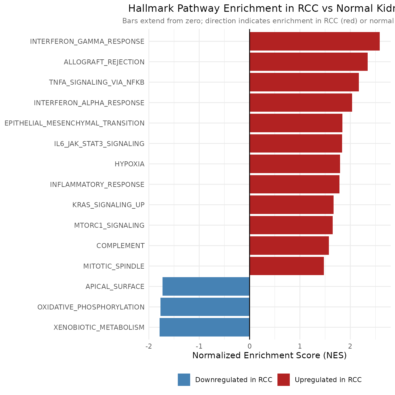
The NES bar chart functions as a part-to-whole visualization at the pathway level: each bar represents one of the 50 Hallmark programs, and the chart as a whole shows the relative contribution of each pathway to the overall transcriptional difference between RCC and normal kidney. The deviation from zero is the central visual encoding, bars extending to the right represent programs activated in RCC, while bars extending to the left represent programs suppressed relative to normal kidney.
The results are strongly consistent with known RCC biology. Pathways with positive NES, enriched among upregulated genes in RCC, are expected to include HYPOXIA, ANGIOGENESIS, GLYCOLYSIS, and MYC_TARGETS, all of which are direct or downstream consequences of constitutive HIF1 activation following VHL loss. Hypoxia response genes are among HIF1’s primary transcriptional targets; angiogenesis is driven by HIF1-induced VEGF secretion; and the metabolic switch to glycolysis (the Warburg effect) is a hallmark of HIF1-active tumors.
Pathways with negative NES, enriched among downregulated genes, are equally revealing. Suppression of OXIDATIVE_PHOSPHORYLATION and FATTY_ACID_METABOLISM pathways is consistent with the metabolic reprogramming of clear cell RCC: the tumor abandons the oxidative metabolism characteristic of the proximal tubule cell of origin in favor of glycolytic energy production. Downregulation of EPITHELIAL_MESENCHYMAL_TRANSITION (if present) would contrast with many other carcinomas and reflect the specific biology of kidney cancer, while suppression of immune pathway gene sets might reflect immune exclusion mechanisms common in RCC.
The leading edge genes, those most responsible for each pathway’s enrichment score, represent the highest-priority candidates for follow-up single-gene analysis and are the most likely to appear in the LASSO biomarker panel in the next section.
11. Promising Trends: Multi-Gene Biomarker Discovery
The final analytical stage asks a translational question: given everything we know about which genes are differentially expressed and which pathways are dysregulated, can a small set of genes serve as a practical diagnostic signature? This is not simply asking which genes are most significant, it is asking which genes carry non-redundant predictive information when considered jointly. This distinction matters enormously in a clinical context, where a 3-gene RT-PCR panel is deployable and a 3,000-gene array is not.
LASSO logistic regression is the appropriate tool for this question.
Applied to the full expression matrix, all ~22,000 probes competing
simultaneously to predict disease state, LASSO shrinks the coefficient
of most genes to exactly zero through L1 regularization, retaining only
those with independent discriminative signal. The penalty strength is
tuned by 10-fold cross-validation, and the final model at
lambda.1se represents the sparsest solution whose
cross-validated accuracy is within one standard error of the optimum, a
deliberate bias toward parsimony that tends to produce more
generalizable panels.
phenotype.binary <- ifelse(geo$phenotype$disease.state == "RCC", 1, 0)
lasso.fit <- fit.lasso(geo$expression, phenotype.binary)

coef.mat <- coef(lasso.fit, s = "lambda.1se")
selected <- coef.mat[coef.mat[, 1] != 0, , drop = FALSE]
n.selected <- nrow(selected) - 1  # subtract intercept

cat("Number of genes selected by LASSO:", n.selected, "\n\n")
#> Number of genes selected by LASSO: 9
print(round(selected, 4))
#> 10 x 1 sparse Matrix of class "dgCMatrix"
#>             lambda.1se
#> (Intercept)     4.5824
#> 222405_at      -0.4997
#> 223798_at       0.5910
#> 226733_at      -0.5953
#> 226851_at      -0.0224
#> 227238_at      -0.0570
#> 227367_at       1.0928
#> 228581_at      -0.4142
#> 229529_at      -0.4307
#> 231391_at      -0.0346
# Visualize the cross-validation curve to show model selection
plot(lasso.fit, main = "LASSO Cross-Validation Curve")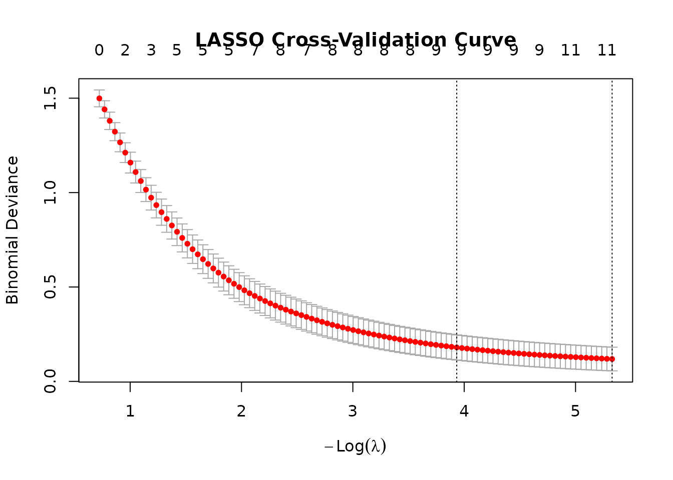
The cross-validation curve plots mean classification error against
the log-regularization penalty (log lambda), with the two vertical
dashed lines marking lambda.min (the penalty minimizing CV
error) and lambda.1se (our chosen, more parsimonious
model). The relatively flat error curve across a range of lambda values
is reassuring, it means the model is not highly sensitive to the exact
penalty chosen, and that the sparse lambda.1se solution
performs nearly as well as the more complex lambda.min
solution.
The LASSO-selected genes represent a candidate diagnostic signature for clear cell RCC. Each selected probe was chosen because it provides classification information not already captured by any other probe in the panel, a form of automatic feature selection that is far more principled than simply taking the top N most significant genes from the limma TopTable. Notably, the selected genes are not necessarily those with the largest individual fold changes. A gene with a moderate fold change but expression highly specific to RCC (low variance in normal tissue) may be more valuable to the classifier than a gene that is more dramatically changed but highly variable across both groups.
Cross-referencing the LASSO-selected probes against the GSEA leading edge genes from Section 10 would identify which pathway members carry the most independent predictive signal, a natural next step for prioritizing genes for experimental validation.
12. Conclusion
This analysis demonstrates that clear cell renal cell carcinoma produces a large, biologically coherent, and statistically robust transcriptional signature relative to normal kidney tissue. The principal findings across the six analytical stages are consistent and mutually reinforcing.
PCA confirmed that disease state is the dominant source of transcriptional variation in the GDS507 dataset, with clean separation of tumor and normal samples along the first principal component. This was a necessary precondition for all subsequent analyses, a dataset dominated by technical noise or batch effects would have required correction before meaningful biological inference was possible.
Genome-wide differential expression analysis identified a large number of significantly dysregulated probe sets at a 5 percent FDR threshold, with asymmetric representation of upregulated versus downregulated genes reflecting both HIF1 pathway activation and the loss of normal proximal tubule cell identity. The interactive volcano plot demonstrated the value of exploratory, hover-capable visualization for high-dimensional genomic data, allowing rapid identification of specific genes of interest without the visual clutter of static label overlays.
Distribution analysis of the top candidates confirmed that the most significant genes show large, consistent effect sizes (Cohen’s d in the large range) that are robust across both parametric and nonparametric tests. The bootstrapped confidence intervals quantify the uncertainty inherent in a 27-sample study and provide an honest basis for interpreting the precision of effect size estimates.
Co-expression analysis revealed coordinated regulatory structure among the top candidates, with clusters of genes sharing expression trajectories consistent with common transcriptional drivers. This structure motivates the LASSO selection in the final stage, tightly co-expressed genes are redundant predictors, and a clinically useful panel must account for this.
Pathway enrichment analysis confirmed the biological coherence of the differential expression signature. The enrichment of hypoxia, angiogenesis, and glycolysis pathways among upregulated genes, and the suppression of oxidative phosphorylation and fatty acid metabolism among downregulated genes, is precisely consistent with constitutive HIF1 activation following VHL loss, the canonical molecular lesion of clear cell RCC. This concordance between data-driven results and prior biological knowledge substantially strengthens confidence in the analytical pipeline.
Finally, LASSO regression identified a sparse gene panel that jointly discriminates RCC from normal tissue. The number of selected genes demonstrates that a small, deployable molecular signature exists within the large differential expression signal, supporting the potential translational utility of expression-based RCC diagnostics.
Several important limitations of this analysis should be acknowledged. The sample size of 27 (17 tumor, 10 normal) is modest for biomarker discovery, and the LASSO cross-validation error estimates will have high variance at this scale. All samples derive from a single study with a single array platform, and the signature has not been validated in an independent cohort, a critical next step before any clinical claims could be made. The analysis also treats RCC as a binary category, ignoring tumor grade, stage, and the molecular heterogeneity within the clear cell subtype that would be relevant for treatment stratification.
Future directions include validation of the LASSO panel in independent GEO datasets (several GDS entries contain RCC expression data), extension to multi-class analysis incorporating papillary and chromophobe RCC subtypes, integration with survival data to identify prognostic rather than diagnostic signatures, and application of the BioUtils framework to RNA-seq data, which has largely superseded microarrays in contemporary transcriptomics but requires additional preprocessing (normalization, variance stabilization) before the same statistical framework can be applied.